Download notebook

Input · EXIOBASE 3.10.1, product-by-product IOT, 2022, with emissions. Question · Which production paths contribute to the selected German final-demand bundle’s combustion CO2 footprint?

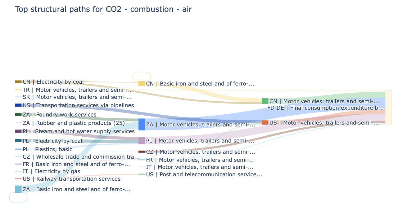
Example output from the companion notebook. Only retained paths are shown; the plot is not the complete footprint.

Analysis steps

1 · Select demand

Parse IOT_2022_pxp.zip. Select Motor vehicles, trailers and semi-trailers (34) and rank its German final-demand categories. The notebook chooses the largest non-zero bundle.

2 · Set the threshold

Calculate the bundle’s total footprint first. The example sets the pruning threshold to 0.1% of its absolute value and explores at most ten upstream rounds.

3 · Trace and inspect

spa = db.calc_spa(
    indicator="CO2 - combustion - air",
    item=SECTOR, final_demand_region=FOCUS_REGION,
    final_demand_category=FOCUS_CATEGORY,
    max_depth=10, cutoff=CUTOFF, top_n=20,
    plot="sankey", show_plot=True,
)
spa.attrs["coverage_share"]

The notebook defines the selectors and CUTOFF in the preceding steps. Compare reported contribution with the full bundle total.

Compare paths with the depth summary

Repeat with top_n=None and plot="depth" to group retained contributions by upstream round. This removes the returned-row cap, but depth and pruning limits still apply.

For a small runnable example, output definitions and limitations, start with Structural path analysis.