Download notebook

Inputs · EXIOBASE monetary product-by-product archives for 2013 and 2014. Item · Nickel ores and concentrates. Outputs · Trade matrices, embodied value added and CO2, concentration and exposure indicators.

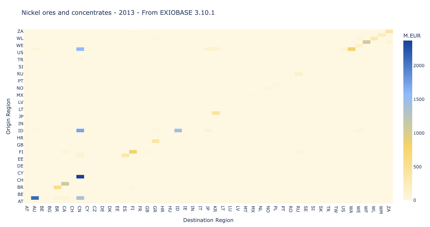
Bilateral trade in the example’s first year. Domestic flows are part of the returned trade matrix.

Analysis steps

1 · Align years

Parse 2013, rename its baseline to "2013", and import 2014 as a second scenario. Keep the same native classification across both.

2 · Locate trade

trade = db.calc_trades(
    item="Nickel ores and concentrates", scenario="2013",
    aggregate=False, total=True,
)

Separate intermediate and final transactions, then compare years or group origin regions into continents.

3 · Attribute impacts

content = db.calc_trades_content(
    indicator="total value added",
    item="Nickel ores and concentrates", scenario="2013",
    method="upstream", breakdown=True,
)

The contributor breakdown identifies production behind each trade pair, beyond the observed exporter.

4 · Measure dependence

Compare concentration across contributors with exposure to a chosen group of regions. Repeat for an available satellite account such as CO2 - combustion - air.

Interpretation: concentrated supply and high exposure answer different questions. Neither measures the absolute size of a flow. Signed indicators need additional care because shares can involve cancellation.

Method definitions and a runnable small example: Trade and supply-chain analysis.